Analyzing Map
What are Vector Symbolic Architectures?
Vector Symbolic Architectures (VSA) are a class of approaches which treat vectors as symbols and use mathematical operators to perform symbolic manipulation on them. Each VSA defines the following:
- A vector sampling distribution $\Omega$
- A binding operator $B(\cdot, \cdot)$
- A bundling operator $+$ (usually addition)
- A retrieval (or unbinding) operator $B^*(\cdot, \cdot)$
To encode information, symbols are bound in key/value (or role/filler) pairs, and then bound pairs are bundled together into a hypervector. Then, using any original key, we can use the retrieval operator to get its corresponding value vector back out of the hypervector.
As an example, consider the sentence “Alex likes chocolate”. We can assign vectors from the VSA’s distribution to the roles $\{First, Second, Third\}$ and values $\{Alex, likes, chocolate\}$.
We can then represent the entire sentence with:
\[S = B(First, Alex) + B(Second, likes) + B(Third, chocolate)\]Then, we can later recover the $First$ word from the sentence with:
\[B^*(S, First) = \widehat{Alex} \approx Alex\]In general, this retrieval process is subject to noise; a “good” VSA is one that is less noisy, in the sense that $\widehat{Alex}$ is very close to $Alex$.
A Motivating Example with Deep Learning
One application of VSAs in deep learning is to compress the size of the (very large) output layer in a neural net being trained for Extreme Multilabel Classification [1], [2]. In such a scenario, the total number of classes $d$ may be so large that the output layer comprises a significant portion of the total weights in the network, while typically only a few labels apply to any given training example [3]. We can use VSAs to convert this into an $n$-dimensional vector regression task, where $n \ll d$.
The scheme proposed by [1] assigns 1 role vector for each class, and two unique filler vectors: $present$ and $absent$. Each training example then constructs a hypervector $S \in \mathbb{R}^n$:
\[S = \underbrace{ \sum_{\mathbf{c}_p \in Y_p} B(present, \mathbf{c}_p) }_{\text{Labels present}} + \underbrace{ \sum_{\mathbf{c}_a \in Y_a} B(absent, \mathbf{c}_a) }_{\text{Labels absent}}\]where $Y_p, Y_a$ are the sets of $present$ and $absent$ role vectors, respectively, for the training example.
The neural net is then trained to produce $S$, from which the predicted present and absent classes are extracted. There are two catches, though. The first is obvious — the scheme only works if you can reliably extract true class labels from $S$, so we’re incentivized to use the best VSA we can find. The second is that you need a way to pick $n$ intelligently — too large, and there’s no reason to use the technique; too small, and retrieval accuracy will suffer. A VSA’s capacity is the number of pairs of vectors it can store without losing retrieval accuracy for a given encoding dimension. Some, like the Holographic Reduced Representation, have theoretical bounds on capacity [4]. Others, such as the Hadamard-derived Linear Binding (HLB), do not.
MAP-I and HLB
MAP – multiply-add-permute – is a family of VSAs which largely share operators, but differ in what distributions they sample vectors from [5], [6].
| VSA | Sampling Distribution | Binding Operator | Bundling Operator | Retrieval Operator |
|---|---|---|---|---|
| MAP-C | $x_i ∼ U (−1, 1)$ | $\odot$ (component-wise multiplication) | $+$ (with cutting) | $\odot$ |
| MAP-B | $x_i ∼ B(1, 0.5) · 2 − 1$ | $\odot$ | $+$ (with thresholding) | $\odot$ |
| MAP-I | $x_i ∼ B(1, 0.5) · 2 − 1$ | $\odot$ | $+$ | $\odot$ |
MAP-I is of particular interest because it can be viewed as a discrete version of HLB as long as you restrict to only ever unbinding using vectors $v \in V^n = \{+1, -1\}^n$ — multiplying and dividing by $\pm 1$ are equivalent, after all.
| VSA | Sampling Distribution | Binding Operator | Bundling Operator | Retrieval Operator |
|---|---|---|---|---|
| HLB | $x_i ∼ \{N(-\mu, 1/d), N(\mu, 1/d) \}$ | $\odot$ | $+$ | $\div$ (component-wise division) |
Since MAP-I is discrete, it has some helpful properties we can use to analyze it. For example, $V^n$ is closed under component-wise multiplication and division, so we have that binding $B: V^n \times V^n \to V^n$
Distance and Dot Products
$V^n$ is a finite set, so there are a finite number of values that dot products can take over its elements. In order to enumerate these dot products, we define the scaled Manhattan distance:
\[d(x, y) = \frac{1}{2} \sum_{i=1}^n |x^{(i)} - y^{(i)}|\]This is equivalent to counting how many elements of $x$ and $y$ are different: if $x_i \neq y_i$, then $\frac{|x_i - y_i|}{2} = 1$. Immediately, we can use this distance formula to say something about dot products between elements of $V^n$:
Lemma 1: $x \cdot y$ is a function of $d(x, y)$ and $n$
$Proof$.
\[x \cdot y = \sum_{i=1}^n x^{(i)}y^{(i)} = \sum_{x^{(i)} = y^{(i)}} x^{(i)}y^{(i)} + \sum_{x^{(i)} \neq y^{(i)}} x^{(i)}y^{(i)} = p - q\]Where $p$ is the number of elements of $x$ and $y$ which are the same, and $q$ is the number of elements of $x$ and $y$ which are different. Therefore, we have $q = d(x, y)$, and $p = n - d(x,y)$. This gives the result
\[x \cdot y = n - 2d(x, y) \tag*{$\blacksquare$}\]Using this lemma, we can describe the probability distribution of dot products over elements of $V^n$. This will be our primary tool for analyzing the capacity of MAP-I.
Corollary 1 - Distribution of Random Dot Products over $V^n$: If $x, y$ are sampled randomly and uniformly from $V^n$, then $x \cdot y = Z ∼ n - 2B(n, 0.5)$. Furthermore, $E[Z] = 0$ $Var[Z] = n$, and
\[P(Z=z) = \frac{ \binom{n}{\frac{n - z}{2}} }{ 2^n }\]$Proof.$
Let $x, y$ be sampled randomly and uniformly from $V^n$, and define $D = d(x, y)$. Consider $x$ “fixed”, and a “successful trial” to be the case that $x^{(i)} = y^{(i)}$. The probability $x^{(i)} = y^{(i)}$ is $50\%$, and $x$ has $n$ elements, so there are $n$ trials. Therefore, $D ∼ B(n, 0.5)$.
Now, let $Z = x \odot y$. Then, by Lemma 1, we also have that
\[Z = n - 2D\]Since $D$ is binomial, we can easily find $E[Z]$ and $Var[Z]$ as well:
\[E[Z] = E[n - 2D] = n - 2E[D] = 0\] \[Var[Z] = Var[n - 2D] = 4Var[D] = n\]Furthermore, we can write $Z$’s PMF explicitly with a simple change of variables:
\[Z = n - 2D \iff D = \frac{n - Z}{2} \implies P(Z=z) = P(D= \frac{n - z}{2}) = \frac{ \binom{n}{\frac{n - z}{2}}}{2^n} \tag*{$\blacksquare$}\]Finally, as our last bit of preparation, we define the vector concatenation operator $\oplus$ and connect it to dot products.
\[\oplus: \mathbb{R}^n \times \mathbb{R}^m \to \mathbb{R}^{n+m}\] \[x \oplus y = \begin{bmatrix} x_1 \\ x_2 \\ \vdots \\ x_n \end{bmatrix} \oplus \begin{bmatrix} y_1 \\ y_2 \\ \vdots \\ y_m \end{bmatrix} = \begin{bmatrix} x_1 \\ \vdots \\ x_n \\ y_1 \\ \vdots \\ y_m \\ \end{bmatrix}\]Lemma 2: $x \cdot y + u \cdot v = x \oplus u \cdot y \oplus v$
$Proof:$
\[x \cdot y + u \cdot v = \sum_{i=1}^n x^{(i)} y^{(i)} + \sum_{j=1}^m u^{(j)} v^{(j)} = \sum_{k=1}^{n+m} (x \oplus u)^{(k)} (y \oplus v)^{(k)}\] \[\text{by definition of vector concatenation.} \tag*{$\blacksquare$}\]Binding and Bundling
Instead of considering binding and bundling as two distinct operations, we’ll consider them as a combined operation over two sets of “left” and “right” vectors.
Let $x_i$, $y_i \in \mathbf{R}^n$, $i=1, 2, \dots, \rho$ be left and right vectors. We’ll organize them into:
\[X = \left(\begin{array}{c|c|c|c} x_1 & x_2 & ... & x_{\rho} \end{array}\right), \quad Y= \left(\begin{array}{c|c|c|c} y_1 & y_2 & ... & y_{\rho} \end{array}\right) \in \mathbb{R}^{n \times \rho}\]Then we define the “bind then bundle” operation $\mathbf{BB}(\cdot, \cdot)$ as
\[\mathbf{BB}(X, Y) = \text{diag}(XY^T) \in \mathbb{R}^n\]There’s a lot of equivalent ways to write that – it’s the same as a componentwise multiplication between the matrices, then summing along the rows. The important thing, however, is that each element of $\mathbf{BB}(X, Y)$ is itself a dot product:
\[\mathbf{BB}(X, Y) = \left( \begin{array}{c} X_1 \cdot Y_1 \\ X_2 \cdot Y_2 \\ \vdots \\ X_n \cdot Y_n \end{array} \right) \quad \text{$X_i,\ Y_i$ are the $i^{th}$ rows of $X$, $Y$, resp.}\]But $X_i$, $Y_i$ are elements of $V^{\rho}$, so their values are distributed according to Corollary 1.
Retrieval
Let $S = \mathbf{BB}(X, Y)$. Given $y$ we want to retrieve $x$ from $S$. We check how good we are at doing this by comparing dot products between the value we unbind $\hat{x} = B^*(S, y)$ and the true result, $x$, giving us a retrieval score $R = \hat{x} \cdot x$. We can split this into two cases. In the “correct” case, we unbind with $y_i$ and take the dot product against $x_i$. Since $x_i$ and $y_i$ are bound together and contained within $S$, we expect the score to be high. In the “incorrect” case we unbind and test with non-matching $x$ and $y$. Since $x$ and $y$ are not bound within $S$, we expect the score to be low. Our goal is to find the PMFs for both of these cases.
First, we have a property of this retrieval process which will simplify things:
Lemma 3: \(B^*(S, y) \cdot x = B^*(S, x) \cdot y\)
$Proof:$
\[B^*(S, y) \cdot x = \sum_{i=1}^n \frac{S^{(i)}}{y^{(i)}} x^{(i)} = \sum_{i=1}^n \frac{S^{(i)}}{x^{(i)}} y^{(i)} = B^*(S, x) \cdot y\] \[\text{because } x^{(i)}, y^{(i)} \in \{-1, +1 \} \tag*{$\blacksquare$}\]Correct Case
For the correct case, we can rewrite $S$:
\[S = \left( \begin{array}{c} x_i^{(1)} \cdot y_i^{(1)} + \alpha_1 \\ x_i^{(2)} \cdot y_i^{(2)} + \alpha_2 \\ \vdots \\ x_i^{(n)} \cdot y_i^{(n)} + \alpha_n \end{array} \right) = \left( \begin{array}{c} x_i^{(1)} \cdot y_i^{(1)} \\ x_i^{(2)} \cdot y_i^{(2)} \\ \vdots \\ x_i^{(n)} \cdot y_i^{(n)} \end{array} \right) + \underbrace{ \left( \begin{array}{c} \alpha_1 \\ \alpha_2 \\ \vdots \\ \alpha_n \end{array} \right) }_{=: \alpha}\]where each $\alpha_i$ is simply the other elements in the sum of the dot product for that entry.
Now, let’s examine $B^*(S, y_i)$:
\[B^*(S, y_i) = S \div y = \left( \begin{array}{c} \frac{x_i^{(1)} \cdot y_i^{(1)}}{y_i} \\ \frac{x_i^{(2)} \cdot y_i^{(2)}}{y_i} \\ \vdots \\ \frac{x_i^{(n)} \cdot y_i^{(n)}}{y_i} \end{array} \right) + \alpha \div y_i = x_i + \alpha \div y_i =: \hat{x}_i\]Now, each $\alpha_k$ is equivalent to a dot product between two random vectors in $V^{\rho-1}$, which means they are random variables following our favorite distribution described above. Accordingly, their distribution is symmetric about $0$, and each $y_i^{(j)}$ is a Rademacher random variable. Therefore the distribution of the random variable $\alpha_k y_i^{(k)}$ is equivalent to $\alpha_k$. In other words, since we already didn’t know the sign of each element of $\alpha$, the fact that it may or may not be swapped by the component-wise division by $y_i^{(k)}$ is irrelevant.
Now, we need to compare $\hat{x}_i$ to $x_i$:
\[\begin{aligned} <\hat{x}_i,\ x_i> & =\ <x_i + \alpha \div y_i,\ x_i> \\ & = <x_i, x_i> + <\alpha \div y_i,\ x_i> \\ & = n + \underbrace{<\alpha \div y_i,\ x_i>}_{=: E} \end{aligned}\]Since $n$ is constant, all we have to do is find the PMF for $E$:
\[E = \sum_{j=1}^n \frac{\alpha_j x_i^{(j)}}{y_i^{(j)}}\]We still have that $x_i^{(j)}$ and $y_i^{(j)}$ are Rademacher random variables, so the PMF of $E$ is equivalent to the PMF of
\[\bar{E} = \sum_{j=1}^n \alpha_j = \sum_{j=1}^n u \cdot w \ \ \ \ \ u, w \in V^{(\rho - 1)}\]Since $\bar{E}$ is the sum of $n$ dot products of vectors in $V^{\rho-1}$, so we can apply Lemma 2 (vector concatenation) to view it as a single $n(\rho-1)$-dimensional dot product over elements of $V^{n(\rho-1)}$. Using Corollary 3, we therefore have that $\bar{E} ∼ B(n (\rho - 1), 0.5)$.
However, we don’t just want the PMF of $E$, we want the PMF of $T = n + E$. Fortunately, this is relatively simple:
\[\begin{aligned} P(T=c) = P(n + E = c) = P(E = c-n) & = \frac{\binom{n(\rho-1)}{(n(\rho-1) - (c-n) ) /2}}{2^{n(\rho-1)}} \\ & = \frac{\binom{n(\rho-1)}{(n\rho -c ) /2}}{2^{n(\rho-1)}} \end{aligned}\]Incorrect Case
The incorrect case is easier. Let $F = B^*(S, y) \cdot x_i$, $y \neq y_i$.
\[B^*(S, y) = S \div y = \left( \begin{array}{c} X_1 \cdot Y_1 \div y^{(1)} \\ X_2 \cdot Y_2 \div y^{(2)} \\ \vdots \\ X_n \cdot Y_n \div y^{(n)} \end{array} \right) = \beta\]Then, like previously, we write $F = \langle \beta, x_i \rangle$ as a sum:
\[F = \sum_{j=1}^n \beta^{(j)} x_i^{(j)} = \sum_{j=1}^n \frac{x_i^{(j)}}{y^{(j)}} X_j \cdot Y_j\]We apply the exact same argument here as we did for $E$ and $\bar{E}$ – the only difference is that we have a sum of $n$ dot products of $\rho$ vectors from $V^\rho$, instead of $\rho-1$. As a result, we get:
\[P(F=c) = \frac{\binom{n\rho}{(n\rho-c)/2}}{2^{n\rho}}\]Charts & Experimental Results
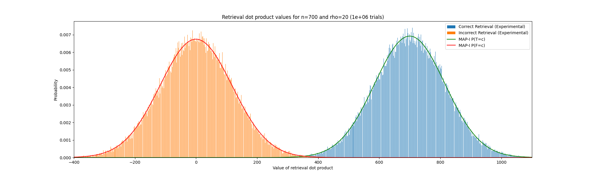
To check the above results, have some charts! For each chart, I computed samples of $T$ and $F$ for a fixed value of $n$ and $\rho$ and plotted the results as a histogram. Separately, I computed the PMFs for $T$ and $F$ using the formulas described above, and overlaid the curves over the histogram.
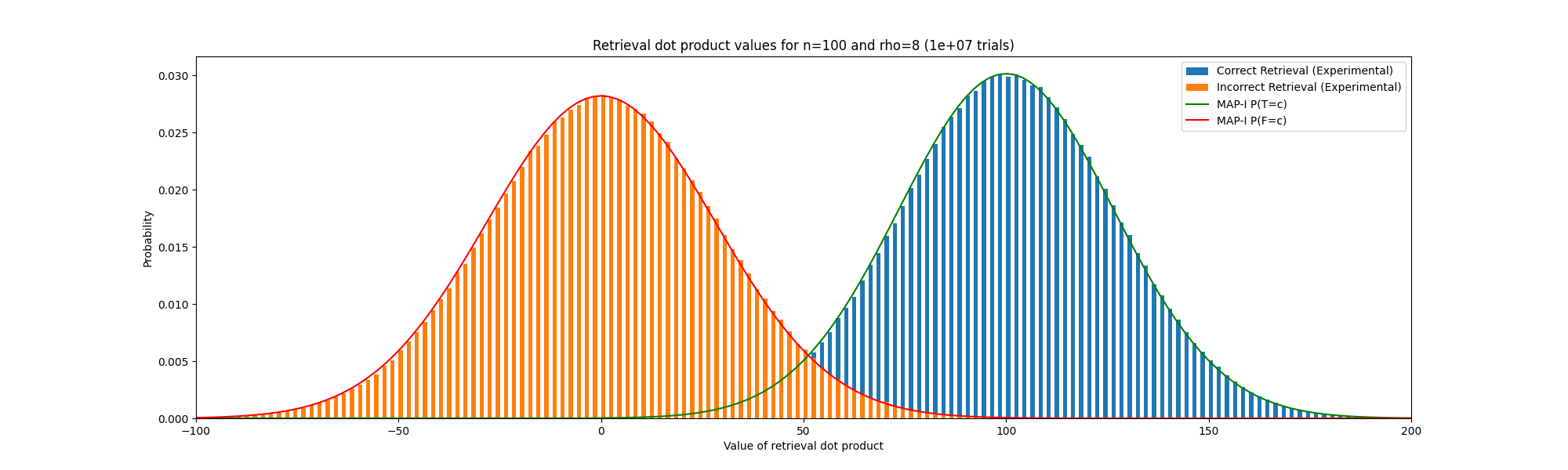
We can see the discrete nature of MAP-I on full display – the histogram has an “empty” space in between each bar. In fact, this is because the parity of $t \sim T$ and $f \sim F$ is determined fully by $n$ and $\rho$. The maximum value of either distribution is $n p$ (in the case that all elements of all vectors bound and bundled into $S$ were equal to $1$), and all possible other values count down by $2$ from there. This does mean the plotted PMFs are slightly dishonest – in reality, they’re not smooth either. However, the plot looks much nicer by pretending they are instead of having them dip back down to $0$ on every other integer, or plotting them as discontinuous line segments.
Separation of Distributions
We can see from the graphs that the distributions for $T$ and $F$ are separated, but that does not tell us by how much. Nor does it tell us in practice how big of a dimension $n$ we need to choose to accurately retrieve from a bundle of $\rho$ pairs. We can use the following inequality to describe what “well separated” means for $T$ and $F$ in terms of their standard deviations:
\[E[T] - a\sqrt{Var[T]} \geq E[F] + a\sqrt{Var[F]} \quad \text{where $a$ is an arbitrary positive constant}\]We can plug in the expected values and variances of $T$ and $F$ using the results from Corollary 1, and solve for $n$ to describe the minimum dimension needed to keep $T$ and $F$ separated by $a$ standard deviations with up to $\rho$ bundled pairs per hypervector:
\[\begin{aligned} & n - a\sqrt{n(\rho-1)} \geq 0 + a\sqrt{n \rho} \\ & \iff n \geq a(\sqrt{n(\rho-1)} + \sqrt{n \rho}) \\ & \iff n^2 \geq a^2(n(\rho-1) + 2\sqrt{n (\rho-1)} \sqrt{n \rho} + n\rho \\ & \iff n^2 \geq a^2(n(\rho-1) + 2n\sqrt{\rho(\rho-1)} + n\rho) \\ & \geq na^2((\rho-1) + 2(\rho-1) + \rho) \\ & \implies n \geq a^2(4\rho - 3) \end{aligned}\]Then solving for $a$, we get the maximum number of standard deviations between the two distributions with given dimension and bundle size:
\[\begin{aligned} & n \geq a^2(4\rho - 3) \\ & \iff a^2 \leq \frac{n}{4\rho-3} \\ & \iff a \leq \sqrt{ \frac{n}{4\rho-3} } \end{aligned}\]These inequalities provide a handy rule of thumb for practitioners seeking to choose an encoding size for their VSAs – choosing $a$ is less explicit than choosing a probability of success, but it is still fairly interpretable. With $a = 3$ or $4$, you can be confident that the distributions will be well separated, and the probability of an incorrect retrieval being mistaken for a correct one is quite low. Additionally, these results align with those recently published in [7]. They experimentally show the same linear relationship between $n$ and $\rho$ for MAP-I, HRR, and HLB that these inequalities prove for MAP-I.
Works Cited
- [1]A. Ganesan et al., “Learning with holographic reduced representations,” Advances in neural information processing systems, vol. 34, pp. 25606–25620, 2021.
- [2]M. M. Alam, A. Oberle, E. Raff, S. Biderman, T. Oates, and J. Holt, “A walsh hadamard derived linear vector symbolic architecture,” Advances in Neural Information Processing Systems, vol. 37, pp. 2711–2733, 2024.
- [3]K. Bhatia et al., “The extreme classification repository: Multi-label datasets and code.” 2016. Available at: http://manikvarma.org/downloads/XC/XMLRepository.html
- [4]T. A. Plate, “Holographic reduced representations,” IEEE Transactions on Neural networks, vol. 6, no. 3, pp. 623–641, 1995.
- [5]R. W. Gayler, “Multiplicative Binding, Representation Operators & Analogy (Workshop Poster).” 1998. Available at: http://cogprints.org/502/
- [6]K. Schlegel, P. Neubert, and P. Protzel, “A comparison of vector symbolic architectures,” Artificial Intelligence Review, vol. 55, no. 6, pp. 4523–4555, Aug. 2022, doi: 10.1007/s10462-021-10110-3.
- [7]F. S. Carzaniga, M. Hersche, K. Schindler, and A. Rahimi, “Practical Lessons on Vector-Symbolic Architectures in Deep Learning-Inspired Environments,” 2025.